When more data makes you more certain of the wrong answer — Astrobytes

Count the stars in a young cluster and sort them by mass. Above roughly a solar mass, the number of stars per unit mass falls off as a power law, $\xi(m) \propto m^{-\alpha}$ . Salpeter measured $\alpha = 2.35$ in 1955, and that one number still does an enormous amount of work: it sets how much of a cluster’s mass ends up in the stars massive enough to ionize their surroundings, drive winds, and explode. Get $\alpha$ wrong and you get the energy budget of a galaxy wrong with it.

So we measure it, carefully, in cluster after cluster. The trouble is what we are actually looking at when we do.

Most massive stars have a companion you cannot see

Stellar multiplicity rises steeply with mass. Roughly a fifth of M dwarfs have a companion; for O stars the fraction approaches 90%.

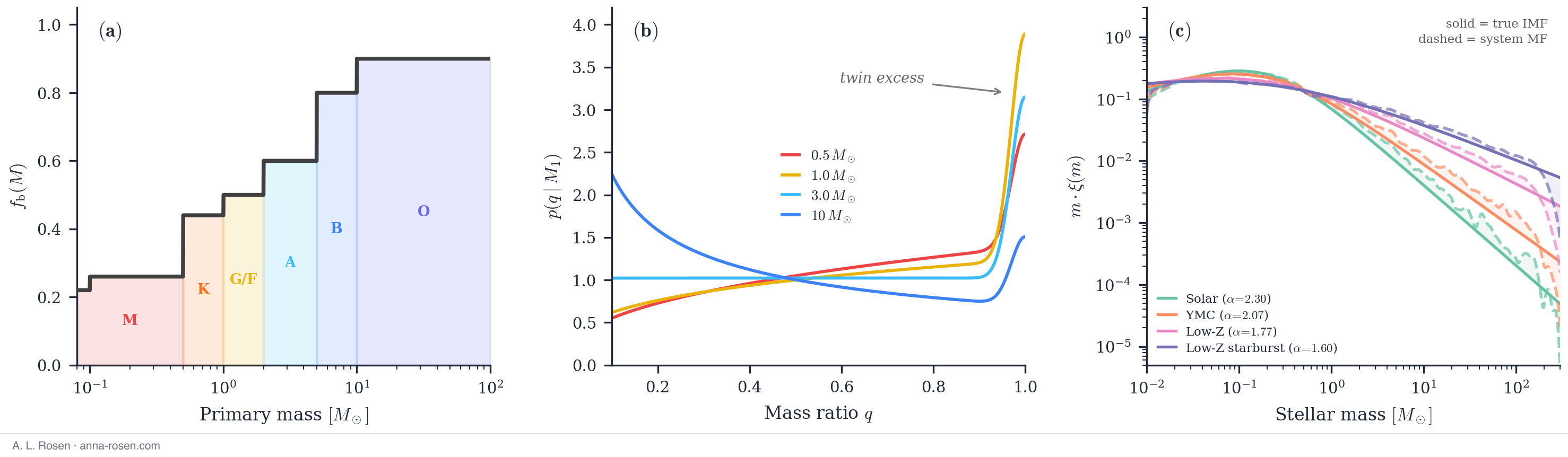
Three panels. (a) Binary fraction as a function of primary mass, rising in steps from about 0.22 for M dwarfs to 0.9 for O stars. (b) Distribution of mass ratio q for four primary masses, showing an excess of near-equal-mass 'twin' pairs at q close to 1. (c) The true initial mass function compared with the system mass function for four environments; the two curves separate at high mass. — The binary population that does the damage. **(a)** The fraction of stars with a companion climbs with primary mass. **(b)** Companions are not drawn uniformly: there is a real excess of near-equal-mass pairs. **(c)** The resulting *system* mass function (dashed) departs from the true IMF (solid) exactly where the high-mass slope is measured.
Figure 1 of Rosen (2026), submitted.

In a photometric survey, an unresolved pair is one point source. You measure one flux, apply a mass–luminosity relation, and record one mass — and that mass is too large, because two stars contributed to it. Every unresolved binary in the sample therefore migrates to higher inferred mass, and the measured high-mass slope comes out shallower than the truth. The bias on $\alpha$ is negative.

How much too large depends on how the pair’s light combines, which depends on the survey. Rather than model one instrument, I bracket the effect with two limiting cases: mass-addition, where the inferred mass is $m_1 + m_2$ , a formal upper bound on the overestimate; and luminosity-addition, where the combined luminosity is inverted through the zero-age main-sequence mass–luminosity relation, an idealized best case for photometry. Real surveys sit between them.

The part that does not go away

Here is the uncomfortable structure of the problem.

The width of your credible interval shrinks as $1/\sqrt{N}$ : measure more stars, and your quoted uncertainty gets smaller, exactly as it should. But this bias is a property of what fraction of your sample is unresolved binaries, not of how many stars you counted. It does not shrink at all.

Two quantities, one falling and one flat, must eventually cross. Past that crossing, the bias is larger than your entire credible interval, and the true value of $\alpha$ sits outside the range you report.

The measurement is precise, and it excludes the right answer. That is the regime I call confidently wrong.

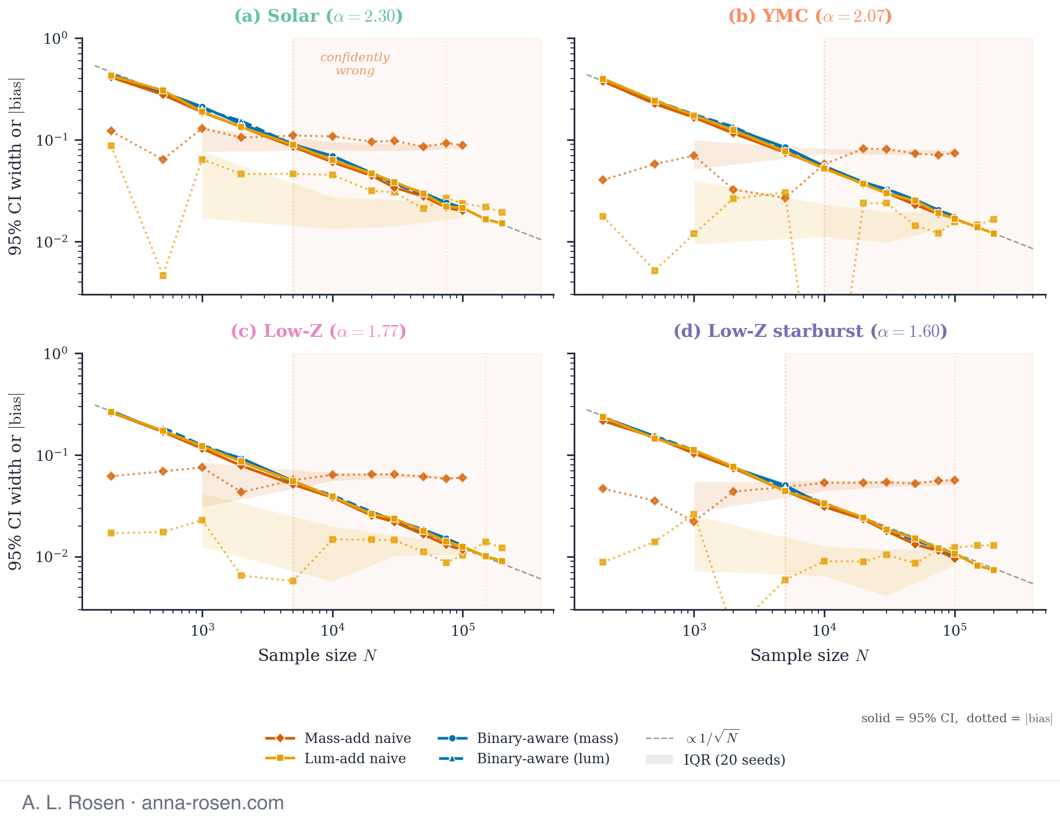
Four log-log panels, one per environment. In each, solid lines showing 95 percent credible-interval width fall along a 1 over root N line, while dotted lines showing absolute bias stay roughly flat. A shaded region marks where the naive bias exceeds the interval width. — Credible-interval width (solid) falls as $1/\sqrt{N}$ ; the bias (dotted) does not fall at all. The shaded region marks where bias exceeds the interval — where the posterior excludes the truth. Binary-aware fits (blue) track the same $1/\sqrt{N}$ scaling, with bias consistent with zero.
Figure 4 of Rosen (2026), submitted.

Across four environments spanning $\alpha = 1.60$ to $2.30$ , the crossover lands at sample sizes we are already reaching:

observation operator	bias in $\alpha$	crossover $N$
mass-addition (upper bound)	0.054–0.086	~5,000–10,000
luminosity-addition (idealized)	0.011–0.021	~75,000–150,000

Gaia, JWST, Roman, and LSST will deliver $10^4$ to $10^6$ resolved stars in a rich cluster. Those sample sizes are not a future problem.

Modeling the binaries fixes it

The fix is not to resolve the companions — you usually cannot — but to stop pretending they are absent. I write a mixture likelihood in which each observed source is either a single star or an unresolved pair, and marginalize over the Moe & Di Stefano (2017) binary population: the mass-dependent multiplicity fraction and mass-ratio distribution in the figure above. The binary content becomes part of the model instead of an unmodeled contaminant.

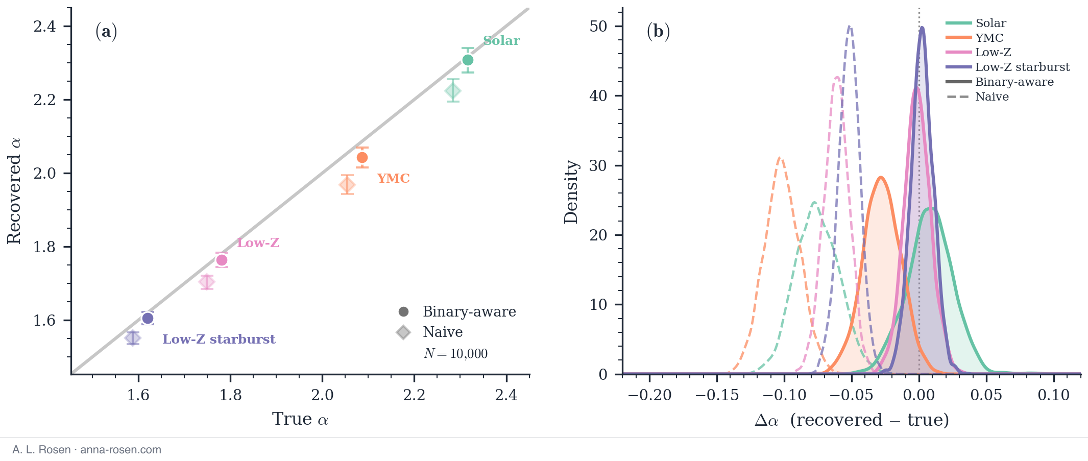
Two panels. Left: recovered versus true slope for four environments; binary-aware estimates lie on the one-to-one line while naive estimates fall below it. Right: posterior distributions of the error; naive posteriors are shifted left of zero, binary-aware posteriors are centred on zero. — Naive fits (dashed, open) sit below the one-to-one line in every environment; binary-aware fits (solid, filled) recover the input slope, with residual posteriors centred on zero.
Figure 3 of Rosen (2026), submitted.

What this means for slopes already in the literature

Published high-mass slopes scatter widely, and that scatter is usually read as genuine environmental variation in the IMF. Some of it may be.

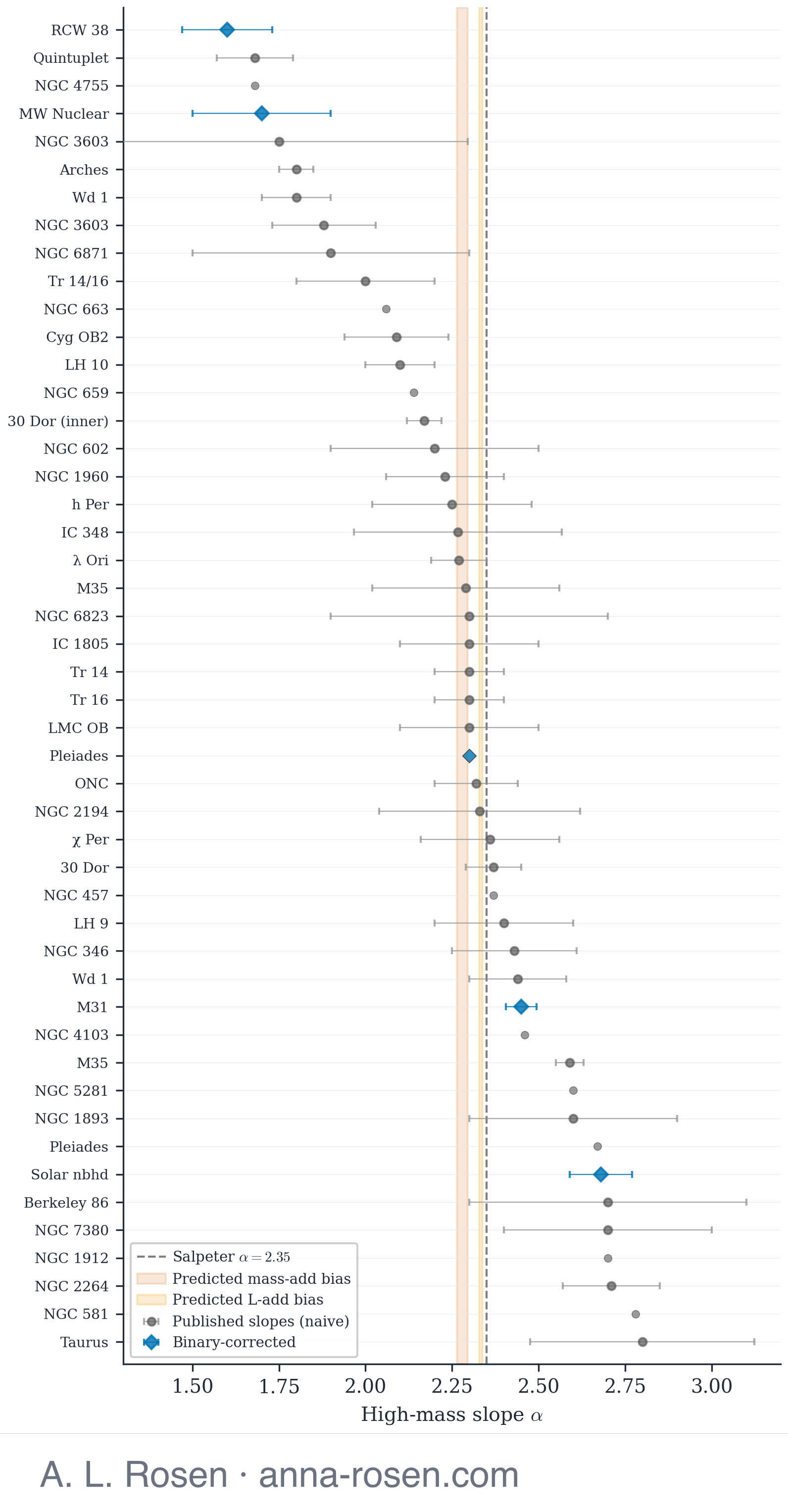
Forest plot of 48 published high-mass IMF slopes with error bars, spanning roughly 1.5 to 2.8, plotted against the Salpeter value of 2.35, with shaded bands marking the predicted bias from mass-addition and luminosity-addition. — 48 published high-mass slopes, against Salpeter (dashed) and the bias predicted here (shaded bands). The offsets this work predicts, 0.01–0.09, are comparable to the error bars many of these measurements carry.
Figure 8 of Rosen (2026), submitted.

But the systematic error predicted here, of order 0.01 to 0.09, is comparable to or larger than the uncertainties quoted on many of these points. That does not make any particular published slope wrong. It does mean that a spread of this size cannot be cleanly attributed to environment until unresolved binaries have been modeled, because a bias of the same magnitude is present whether or not the IMF itself varies.

What this does not show

These are controlled experiments on synthetic populations, not a reanalysis of any real cluster. The two observation operators bracket the effect; neither reproduces the selection function, crowding, or photometric errors of a specific survey. And the recovery relies on the binary statistics being approximately those of Moe & Di Stefano — if a cluster’s multiplicity differs substantially, the correction inherits that error.

What survives all of that is the scaling argument, and it does not depend on the details: any bias that stays constant while your error bars shrink will eventually dominate them. The useful question for the coming surveys is not whether they will measure $\alpha$ precisely. They will. It is whether the number they converge on is the right one.